Project FOMC4263 services include NGS sequencing of the V1V3 region of the 16S rRNA amplicons from the samples. First and foremost, please
download this report, as well as the sequence raw data from the download links provided below.
These links will expire after 60 days. We cannot guarantee the availability of your data after 60 days.
Bioinformatics analysis service was not requested, however we still provide the sequence data quality trimming, noise-filtering, pair merging, as well as chimera filtering for the sequences, using the
DADA2 denoising algorithm and pipeline. The denoised, merged and chimera-free ASV (amplicon sequence variants) sequences allow you to perform
downstream analyses such as taxonomy assignment, diversity analysis and differential abundance analysis. If you need us help with these downstream bioinformatics analysis please contact us.
The samples were processed and analyzed with the ZymoBIOMICS® Service: Targeted
Metagenomic Sequencing (Zymo Research, Irvine, CA).
DNA Extraction: If DNA extraction was performed, one of three different DNA
extraction kits was used depending on the sample type and sample volume and were
used according to the manufacturer’s instructions, unless otherwise stated. The kit used
in this project is marked below:
☐
ZymoBIOMICS® DNA Miniprep Kit (Zymo Research, Irvine, CA)
☐
ZymoBIOMICS® DNA Microprep Kit (Zymo Research, Irvine, CA)
☐
ZymoBIOMICS®-96 MagBead DNA Kit (Zymo Research, Irvine, CA)
☑
N/A (DNA Extraction Not Performed)
Elution Volume: 50µL
Additional Notes: NA
Targeted Library Preparation: The DNA samples were prepared for targeted
sequencing with the Quick-16S™ NGS Library Prep Kit (Zymo Research, Irvine, CA).
These primers were custom designed by Zymo Research to provide the best coverage
of the 16S gene while maintaining high sensitivity. The primer sets used in this project
are marked below:
☐
Quick-16S™ Primer Set V1-V2 (Zymo Research, Irvine, CA)
☑
Quick-16S™ Primer Set V1-V3 (Zymo Research, Irvine, CA)
☑
Quick-16S™ Primer Set V3-V4 (Zymo Research, Irvine, CA)
☐
Quick-16S™ Primer Set V4 (Zymo Research, Irvine, CA)
☐
Quick-16S™ Primer Set V6-V8 (Zymo Research, Irvine, CA)
☐
Other: NA
Additional Notes: NA
The sequencing library was prepared using an innovative library preparation process in
which PCR reactions were performed in real-time PCR machines to control cycles and
therefore limit PCR chimera formation. The final PCR products were quantified with
qPCR fluorescence readings and pooled together based on equal molarity. The final
pooled library was cleaned up with the Select-a-Size DNA Clean & Concentrator™
(Zymo Research, Irvine, CA), then quantified with TapeStation® (Agilent Technologies,
Santa Clara, CA) and Qubit® (Thermo Fisher Scientific, Waltham, WA).
Control Samples: The ZymoBIOMICS® Microbial Community Standard (Zymo
Research, Irvine, CA) was used as a positive control for each DNA extraction, if
performed. The ZymoBIOMICS® Microbial Community DNA Standard (Zymo Research,
Irvine, CA) was used as a positive control for each targeted library preparation.
Negative controls (i.e. blank extraction control, blank library preparation control) were
included to assess the level of bioburden carried by the wet-lab process.
Sequencing: The final library was sequenced on Illumina® MiSeq™ with a V3 reagent kit
(600 cycles). The sequencing was performed with 10% PhiX spike-in.
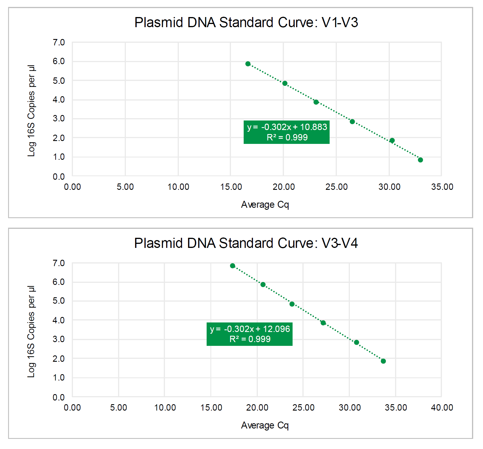
Absolute Abundance Quantification*: A quantitative real-time PCR was set up with a
standard curve. The standard curve was made with plasmid DNA containing one copy
of the 16S gene and one copy of the fungal ITS2 region prepared in 10-fold serial
dilutions. The primers used were the same as those used in Targeted Library
Preparation. The equation generated by the plasmid DNA standard curve was used to
calculate the number of gene copies in the reaction for each sample. The PCR input
volume (2 µl) was used to calculate the number of gene copies per microliter in each
DNA sample.
The number of genome copies per microliter DNA sample was calculated by dividing
the gene copy number by an assumed number of gene copies per genome. The value
used for 16S copies per genome is 4. The value used for ITS copies per genome is 200.
The amount of DNA per microliter DNA sample was calculated using an assumed
genome size of 4.64 x 10⁶ bp, the genome size of Escherichia coli, for 16S samples, or
an assumed genome size of 1.20 x 10⁷ bp, the genome size of Saccharomyces
cerevisiae, for ITS samples. This calculation is shown below:
Calculated Total DNA = Calculated Total Genome Copies × Assumed Genome Size (4.64 × 10⁶ bp) ×
Average Molecular Weight of a DNA bp (660 g/mole/bp) ÷ Avogadro’s Number (6.022 x 10²³/mole)
* Absolute Abundance Quantification is only available for 16S and ITS analyses.
The absolute abundance standard curve data can be viewed in Excel here:
The absolute abundance standard curve is shown below:
The complete report of your project, including all links in this report, can be downloaded by clicking the link provided below. The downloaded file is a compressed ZIP file and once unzipped, open the file “REPORT.html” (may only shown as "REPORT" in your computer) by double clicking it. Your default web browser will open it and you will see the exact content of this report.
Please download and save the file to your computer storage device. The download link will expire after 60 days upon your receiving of this report.
Complete report download link:
To view the report, please follow the following steps:
1.
Download the .zip file from the report link above.
2.
Extract all the contents of the downloaded .zip file to your desktop.
3.
Open the extracted folder and find the "REPORT.html" (may shown as only "REPORT").
4.
Open (double-clicking) the REPORT.html file. Your default browser will open the top age of the complete report. Within the
report, there are links to view all the analyses performed for the project.
The raw NGS sequence data is available for download with the link provided below. The data is a compressed ZIP file and can be unzipped to individual sequence files.
Since this is a pair-end sequencing, each of your samples is represented by two sequence files, one for READ 1,
with the file extension “*_R1.fastq.gz”, another READ 2, with the file extension “*_R1.fastq.gz”.
The files are in FASTQ format and are compressed. FASTQ format is a text-based data format for storing both a biological sequence
and its corresponding quality scores. Most sequence analysis software will be able to open them.
The Sample IDs associated with the R1 and R2 fastq files are listed in the table below:
Sample ID
Read 1 File Name
Read 2 File Name
FOMC4263.Sample1V1V3
zr4263_1V1V3_R1.fastq.gz
zr4263_1V1V3_R2.fastq.gz
FOMC4263.Sample1V3V4
zr4263_1V3V4_R1.fastq.gz
zr4263_1V3V4_R2.fastq.gz
FOMC4263.Sample2V1V3
zr4263_2V1V3_R1.fastq.gz
zr4263_2V1V3_R2.fastq.gz
FOMC4263.Sample2V3V4
zr4263_2V3V4_R1.fastq.gz
zr4263_2V3V4_R2.fastq.gz
Please download and save the file to your computer storage device. The download link will expire after 60 days upon your receiving of this report.
DADA2 is a software package that models and corrects Illumina-sequenced amplicon errors.
DADA2 infers sample sequences exactly, without coarse-graining into OTUs,
and resolves differences of as little as one nucleotide. DADA2 identified more real variants
and output fewer spurious sequences than other methods.
DADA2’s advantage is that it uses more of the data. The DADA2 error model incorporates quality information,
which is ignored by all other methods after filtering. The DADA2 error model incorporates quantitative abundances,
whereas most other methods use abundance ranks if they use abundance at all.
The DADA2 error model identifies the differences between sequences, eg. A->C,
whereas other methods merely count the mismatches. DADA2 can parameterize its error model from the data itself,
rather than relying on previous datasets that may or may not reflect the PCR and sequencing protocols used in your study.
DADA2 pipeline includes several tools for read quality control, including quality filtering, trimming, denoising, pair merging and chimera filtering. Below are the major processing steps of DADA2:
Step 1. Read trimming based on sequence quality
The quality of NGS Illumina sequences often decreases toward the end of the reads.
DADA2 allows to trim off the poor quality read ends in order to improve the error
model building and pair mergicing performance.
Step 2. Learn the Error Rates
The DADA2 algorithm makes use of a parametric error model (err) and every
amplicon dataset has a different set of error rates. The learnErrors method
learns this error model from the data, by alternating estimation of the error
rates and inference of sample composition until they converge on a jointly
consistent solution. As in many machine-learning problems, the algorithm must
begin with an initial guess, for which the maximum possible error rates in
this data are used (the error rates if only the most abundant sequence is
correct and all the rest are errors).
Step 3. Infer amplicon sequence variants (ASVs) based on the error model built in previous step. This step is also called sequence "denoising".
The outcome of this step is a list of ASVs that are the equivalent of oligonucleotides.
Step 4. Merge paired reads. If the sequencing products are read pairs, DADA2 will merge the R1 and R2 ASVs into single sequences.
Merging is performed by aligning the denoised forward reads with the reverse-complement of the corresponding
denoised reverse reads, and then constructing the merged “contig” sequences.
By default, merged sequences are only output if the forward and reverse reads overlap by
at least 12 bases, and are identical to each other in the overlap region (but these conditions can be changed via function arguments).
Step 5. Remove chimera.
The core dada method corrects substitution and indel errors, but chimeras remain. Fortunately, the accuracy of sequence variants
after denoising makes identifying chimeric ASVs simpler than when dealing with fuzzy OTUs.
Chimeric sequences are identified if they can be exactly reconstructed by
combining a left-segment and a right-segment from two more abundant “parent” sequences. The frequency of chimeric sequences varies substantially
from dataset to dataset, and depends on on factors including experimental procedures and sample complexity.
Results
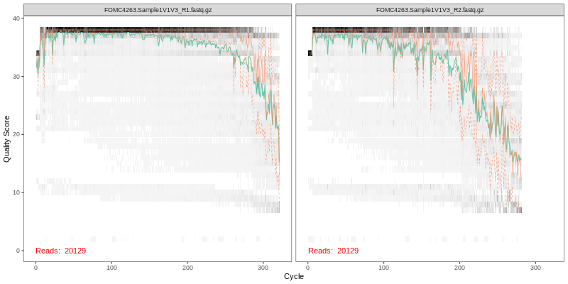
1. Read Quality Plots NGS sequence analaysis starts with visualizing the quality of the sequencing. Below are the quality plots of the first
sample for the R1 and R2 reads separately. In gray-scale is a heat map of the frequency of each quality score at each base position. The mean
quality score at each position is shown by the green line, and the quartiles of the quality score distribution by the orange lines.
The forward reads are usually of better quality. It is a common practice to trim the last few nucleotides to avoid less well-controlled errors
that can arise there. The trimming affects the downstream steps including error model building, merging and chimera calling. FOMC uses an empirical
approach to test many combinations of different trim length in order to achieve best final amplicon sequence variants (ASVs), see the next
section “Optimal trim length for ASVs”.
Below is the link to a PDF file for viewing the quality plots for all samples:
2. Optimal trim length for ASVs The final number of merged and chimera-filtered ASVs depends on the quality filtering (hence trimming) in the very beginning of the DADA2 pipeline.
In order to achieve highest number of ASVs, an empirical approach was used -
Create a random subset of each sample consisting of 5,000 R1 and 5,000 R2 (to reduce computation time)
Trim 10 bases at a time from the ends of both R1 and R2 up to 50 bases
For each combination of trimmed length (e.g., 300x300, 300x290, 290x290 etc), the trimmed reads are
subject to the entire DADA2 pipeline for chimera-filtered merged ASVs
The combination with highest percentage of the input reads becoming final ASVs is selected for the complete set of data
Below is the result of such operation, showing ASV percentages of total reads for all trimming combinations (1st Column = R1 lengths in bases; 1st Row = R2 lengths in bases):
R1/R2
281
271
261
251
241
231
321
34.53%
59.73%
59.23%
56.67%
52.70%
45.81%
311
41.62%
67.67%
66.72%
65.92%
60.10%
56.52%
301
41.01%
69.50%
69.50%
65.00%
59.79%
57.97%
291
39.27%
67.55%
65.97%
63.89%
58.56%
51.77%
281
40.73%
66.27%
66.89%
65.11%
55.59%
40.85%
271
40.28%
66.23%
65.17%
58.12%
39.27%
39.33%
Based on the above result, the trim length combination of R1 = 301 bases and R2 = 271 bases (highlighted red above), was chosen for generating final ASVs for all sequences.
This combination generated highest number of merged non-chimeric ASVs and was used for downstream analyses, if requested.
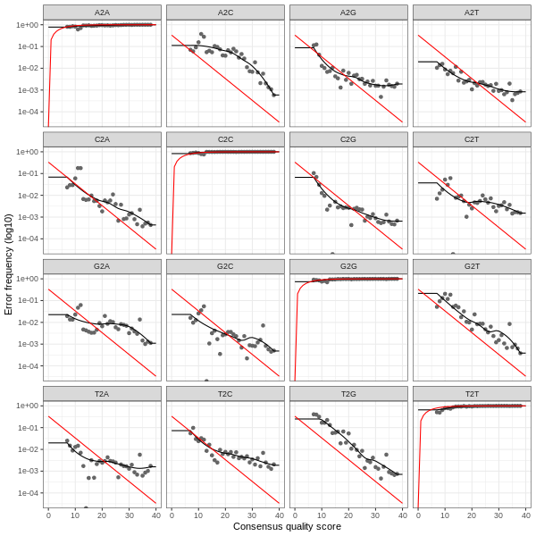
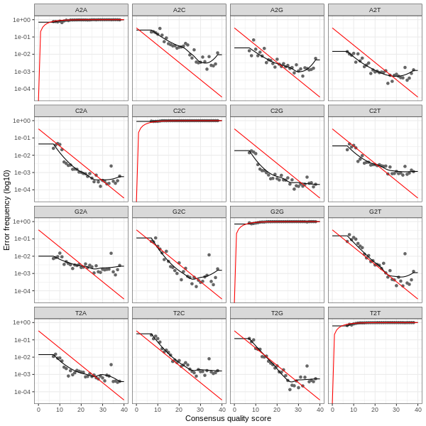
3. Error plots from learning the error rates
After DADA2 building the error model for the set of data, it is always worthwhile, as a sanity check if nothing else, to visualize the estimated error rates.
The error rates for each possible transition (A→C, A→G, …) are shown below. Points are the observed error rates for each consensus quality score.
The black line shows the estimated error rates after convergence of the machine-learning algorithm.
The red line shows the error rates expected under the nominal definition of the Q-score.
The ideal result would be the estimated error rates (black line) are a good fit to the observed rates (points), and the error rates drop
with increased quality as expected.
Forward Read R1 Error Plot
Reverse Read R2 Error Plot
The PDF version of these plots are available here:
4. DADA2 Result Summary The table below shows the summary of the DADA2 analysis,
tracking paired read counts of each samples for all the steps during DADA2 denoising process -
including end-trimming (filtered), denoising (denoisedF, denoisedF), pair merging (merged) and chimera removal (nonchim).
Sample ID
FOMC4263.Sample1V1V3
FOMC4263.Sample1V3V4
FOMC4263.Sample2V1V3
FOMC4263.Sample2V3V4
Row Sum
Percentage
input
20,129
34,970
38,328
33,488
126,915
100.00%
filtered
7,844
24,926
9,398
17,849
60,017
47.29%
denoisedF
7,776
23,885
9,250
17,590
58,501
46.09%
denoisedR
7,705
24,198
9,264
17,290
58,457
46.06%
merged
7,462
23,008
8,981
17,001
56,452
44.48%
nonchim
4,469
8,347
4,790
3,185
20,791
16.38%
This table can be downloaded as an Excel table below:
5. DADA2 Amplicon Sequence Variants (ASVs). A total of 632 unique merged and chimera-free ASV sequences were identified, and their corresponding
read counts for each sample are available in the "ASV Read Count Table" with rows for the ASV sequences and columns for sample. This read count table can be used for
microbial profile comparison among different samples and the sequences provided in the table can be used to taxonomy assignment.
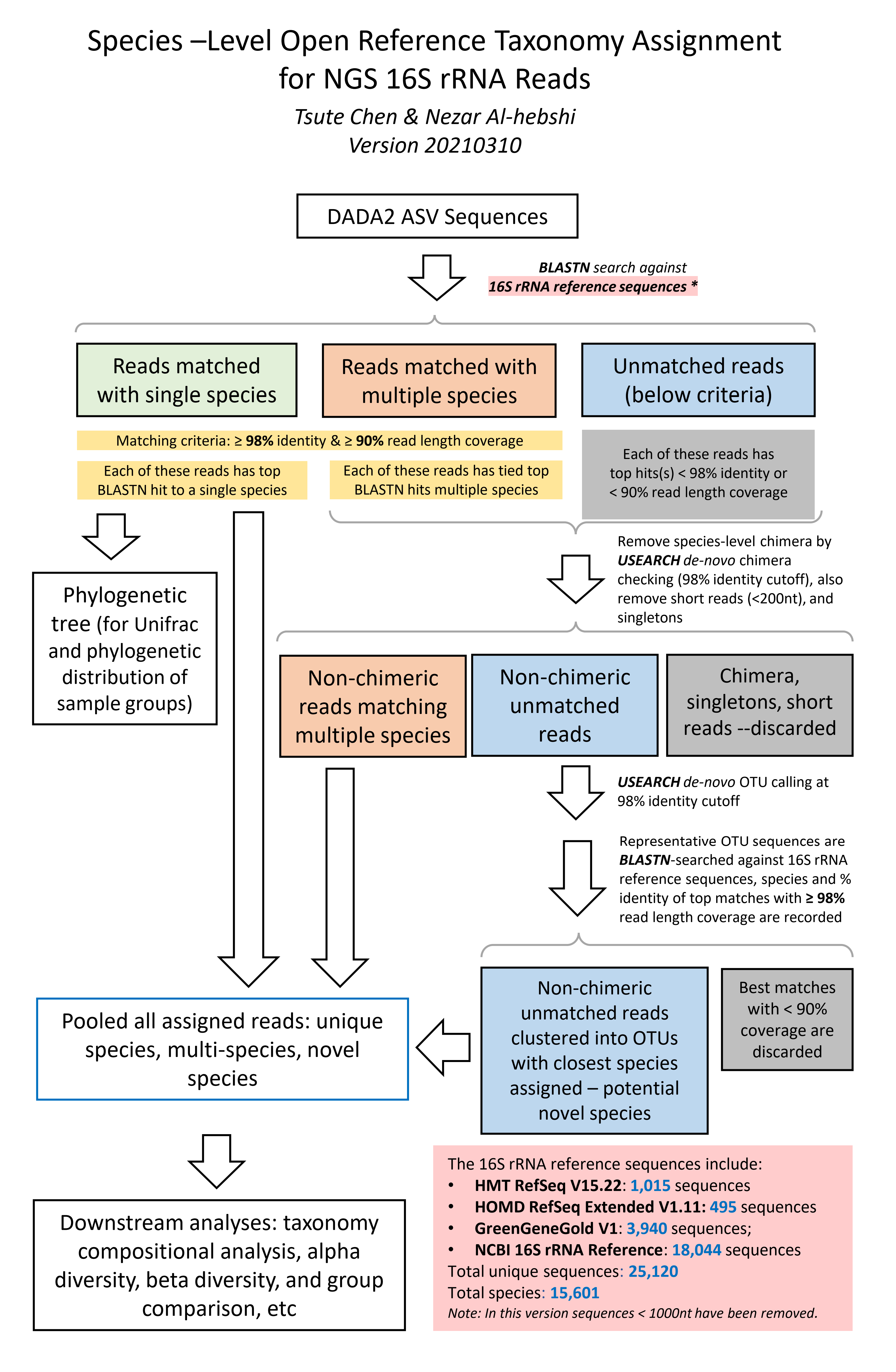
The species-level, open-reference 16S rRNA NGS reads taxonomy assignment pipeline
Version 20210310
1. Raw sequences reads in FASTA format were BLASTN-searched against a combined set of 16S rRNA reference sequences.
It consists of MOMD (version 0.1), the HOMD (version 15.2 http://www.homd.org/index.php?name=seqDownload&file&type=R ),
HOMD 16S rRNA RefSeq Extended Version 1.1 (EXT), GreenGene Gold (GG)
(http://greengenes.lbl.gov/Download/Sequence_Data/Fasta_data_files/gold_strains_gg16S_aligned.fasta.gz) ,
and the NCBI 16S rRNA reference sequence set (https://ftp.ncbi.nlm.nih.gov/blast/db/16S_ribosomal_RNA.tar.gz).
These sequences were screened and combined to remove short sequences (<1000nt), chimera, duplicated and sub-sequences,
as well as sequences with poor taxonomy annotation (e.g., without species information).
This process resulted in 1,015 from HOMD V15.22, 495 from EXT, 3,940 from GG and 18,044 from NCBI, a total of 25,120 sequences.
Altogether these sequence represent a total of 15,601 oral and non-oral microbial species.
The NCBI BLASTN version 2.7.1+ (Zhang et al, 2000) was used with the default parameters.
Reads with ≥ 98% sequence identity to the matched reference and ≥ 90% alignment length
(i.e., ≥ 90% of the read length that was aligned to the reference and was used to calculate
the sequence percent identity) were classified based on the taxonomy of the reference sequence
with highest sequence identity. If a read matched with reference sequences representing
more than one species with equal percent identity and alignment length, it was subject
to chimera checking with USEARCH program version v8.1.1861 (Edgar 2010). Non-chimeric reads with multi-species
best hits were considered valid and were assigned with a unique species
notation (e.g., spp) denoting unresolvable multiple species.
2. Unassigned reads (i.e., reads with < 98% identity or < 90% alignment length) were pooled together and reads < 200 bases were
removed. The remaining reads were subject to the de novo
operational taxonomy unit (OTU) calling and chimera checking using the USEARCH program version v8.1.1861 (Edgar 2010).
The de novo OTU calling and chimera checking was done using 98% as the sequence identity cutoff, i.e., the species-level OTU.
The output of this step produced species-level de novo clustered OTUs with 98% identity.
Representative reads from each of the OTUs/species were then BLASTN-searched
against the same reference sequence set again to determine the closest species for
these potential novel species. These potential novel species were pooled together with the reads that were signed to specie-level in
the previous step, for down-stream analyses.
Reference:
Edgar RC. Search and clustering orders of magnitude faster than BLAST.
Bioinformatics. 2010 Oct 1;26(19):2460-1. doi: 10.1093/bioinformatics/btq461. Epub 2010 Aug 12. PubMed PMID: 20709691.
3. Designations used in the taxonomy:
	1) Taxonomy levels are indicated by these prefixes:

	   k__: domain/kingdom
	   p__: phylum
	   c__: class
	   o__: order
	   f__: family
	   g__: genus
	   s__: species

	   Example:

	   k__Bacteria;p__Firmicutes;c__Clostridia;o__Clostridiales;f__Lachnospiraceae;g__Blautia;s__faecis

	2) Unique level identified – known species:

	   k__Bacteria;p__Firmicutes;c__Clostridia;o__Clostridiales;f__Lachnospiraceae;g__Roseburia;s__hominis

	   The above example shows some reads match to a single species (all levels are unique)

	3) Non-unique level identified – known species:

	   k__Bacteria;p__Firmicutes;c__Clostridia;o__Clostridiales;f__Lachnospiraceae;g__Roseburia;s__multispecies_spp123_3

	   The above example “s__multispecies_spp123_3” indicates certain reads equally match to 3 species of the
	   genus Roseburia; the “spp123” is a temporally assigned species ID.

	   k__Bacteria;p__Firmicutes;c__Clostridia;o__Clostridiales;f__Lachnospiraceae;g__multigenus;s__multispecies_spp234_5

	   The above example indicates certain reads match equally to 5 different species, which belong to multiple genera.;
	   the “spp234” is a temporally assigned species ID.

	4) Unique level identified – unknown species, potential novel species:

	   k__Bacteria;p__Firmicutes;c__Clostridia;o__Clostridiales;f__Lachnospiraceae;g__Roseburia;s__ hominis_nov_97%

	   The above example indicates that some reads have no match to any of the reference sequences with
	   sequence identity ≥ 98% and percent coverage (alignment length)  ≥ 98% as well. However this groups
	   of reads (actually the representative read from a de novo  OTU) has 96% percent identity to
	   Roseburia hominis, thus this is a potential novel species, closest to Roseburia hominis.
	   (But they are not the same species).

	5) Multiple level identified – unknown species, potential novel species:
	   k__Bacteria;p__Firmicutes;c__Clostridia;o__Clostridiales;f__Lachnospiraceae;g__Roseburia;s__ multispecies_sppn123_3_nov_96%

	   The above example indicates that some reads have no match to any of the reference sequences
	   with sequence identity ≥ 98% and percent coverage (alignment length)  ≥ 98% as well.
	   However this groups of reads (actually the representative read from a de novo  OTU)
	   has 96% percent identity equally to 3 species in Roseburia. Thus this is no single
	   closest species, instead this group of reads match equally to multiple species at 96%.
	   Since they have passed chimera check so they represent a novel species. “sppn123” is a
	   temporary ID for this potential novel species.
4. The taxonomy assignment algorithm is illustrated in this flow char below:
Read Taxonomy Assignment - Result Summary
Code
Category
Read Count (MC=1)*
Read Count (MC=100)*
A
Total reads
20,791
20,791
B
Total assigned reads
20,684
20,684
C
Assigned reads in species with read count < MC
0
1,027
D
Assigned reads in samples with read count < 500
0
0
E
Total samples
4
4
F
Samples with reads >= 500
4
4
G
Samples with reads < 500
0
0
H
Total assigned reads used for analysis (B-C-D)
20,684
19,657
I
Reads assigned to single species
15,037
14,564
J
Reads assigned to multiple species
3,606
3,295
K
Reads assigned to novel species
2,041
1,798
L
Total number of species
65
40
M
Number of single species
33
26
N
Number of multi-species
14
9
O
Number of novel species
18
5
P
Total unassigned reads
107
107
Q
Chimeric reads
0
0
R
Reads without BLASTN hits
54
54
S
Others: short, low quality, singletons, etc.
53
53
A=B+P=C+D+H+Q+R+S
E=F+G
B=C+D+H
H=I+J+K
L=M+N+O
P=Q+R+S
* MC = Minimal Count per species, species with total read count < MC were removed.
* The assignment result from MC=100 was used in the downstream analyses.
Read Taxonomy Assignment - Sample Meta Information
#SampleID
Group
FOMC4263.Sample1V1V3
V1V3
FOMC4263.Sample1V3V4
V3V4
FOMC4263.Sample2V1V3
V1V3
FOMC4263.Sample2V3V4
V3V4
Read Taxonomy Assignment - ASV Read Counts by Samples