Project FOMC4799 services include NGS sequencing of the V3V4 region of the 16S rRNA amplicons from the samples. First and foremost, please download this report, as well as the sequence raw data from the download links provided below. These links will expire after 60 days. We cannot guarantee the availability of your data after 60 days.

Bioinformatics analysis service was not requested, however we still provide the sequence data quality trimming, noise-filtering, pair merging, as well as chimera filtering for the sequences, using the DADA2 denoising algorithm and pipeline. The denoised, merged and chimera-free ASV (amplicon sequence variants) sequences allow you to perform downstream analyses such as taxonomy assignment, diversity analysis and differential abundance analysis. If you need us help with these downstream bioinformatics analysis please contact us.

The samples were processed and analyzed with the ZymoBIOMICS® Service: Targeted Metagenomic Sequencing (Zymo Research, Irvine, CA).

DNA Extraction: If DNA extraction was performed, one of three different DNA extraction kits was used depending on the sample type and sample volume and were used according to the manufacturer’s instructions, unless otherwise stated. The kit used in this project is marked below:

Targeted Library Preparation: The DNA samples were prepared for targeted sequencing with the Quick-16S™ NGS Library Prep Kit (Zymo Research, Irvine, CA). These primers were custom designed by Zymo Research to provide the best coverage of the 16S gene while maintaining high sensitivity. The primer sets used in this project are marked below:

The sequencing library was prepared using an innovative library preparation process in which PCR reactions were performed in real-time PCR machines to control cycles and therefore limit PCR chimera formation. The final PCR products were quantified with qPCR fluorescence readings and pooled together based on equal molarity. The final pooled library was cleaned up with the Select-a-Size DNA Clean & Concentrator™ (Zymo Research, Irvine, CA), then quantified with TapeStation® (Agilent Technologies, Santa Clara, CA) and Qubit® (Thermo Fisher Scientific, Waltham, WA).

Control Samples: The ZymoBIOMICS® Microbial Community Standard (Zymo Research, Irvine, CA) was used as a positive control for each DNA extraction, if performed. The ZymoBIOMICS® Microbial Community DNA Standard (Zymo Research, Irvine, CA) was used as a positive control for each targeted library preparation. Negative controls (i.e. blank extraction control, blank library preparation control) were included to assess the level of bioburden carried by the wet-lab process.

Sequencing: The final library was sequenced on Illumina® MiSeq™ with a V3 reagent kit (600 cycles). The sequencing was performed with 10% PhiX spike-in.

The complete report of your project, including all links in this report, can be downloaded by clicking the link provided below. The downloaded file is a compressed ZIP file and once unzipped, open the file “REPORT.html” (may only shown as "REPORT" in your computer) by double clicking it. Your default web browser will open it and you will see the exact content of this report.

Please download and save the file to your computer storage device. The download link will expire after 60 days upon your receiving of this report.

Complete report download link:

To view the report, please follow the following steps:

1.	Download the .zip file from the report link above.
2.	Extract all the contents of the downloaded .zip file to your desktop.
3.	Open the extracted folder and find the "REPORT.html" (may shown as only "REPORT").
4.	Open (double-clicking) the REPORT.html file. Your default browser will open the top age of the complete report. Within the report, there are links to view all the analyses performed for the project.

The raw NGS sequence data is available for download with the link provided below. The data is a compressed ZIP file and can be unzipped to individual sequence files. Since this is a pair-end sequencing, each of your samples is represented by two sequence files, one for READ 1, with the file extension “*_R1.fastq.gz”, another READ 2, with the file extension “*_R1.fastq.gz”. The files are in FASTQ format and are compressed. FASTQ format is a text-based data format for storing both a biological sequence and its corresponding quality scores. Most sequence analysis software will be able to open them. The Sample IDs associated with the R1 and R2 fastq files are listed in the table below:

Sample ID
Original Sample ID
Read 1 File Name
Read 2 File Name
S01
1AB
zr4799_10V3V4_R1.fastq.gz
zr4799_10V3V4_R2.fastq.gz
S02
2AB
zr4799_11V3V4_R1.fastq.gz
zr4799_11V3V4_R2.fastq.gz
S03
3AB
zr4799_12V3V4_R1.fastq.gz
zr4799_12V3V4_R2.fastq.gz
S04
4AB
zr4799_13V3V4_R1.fastq.gz
zr4799_13V3V4_R2.fastq.gz
S05
5AB
zr4799_14V3V4_R1.fastq.gz
zr4799_14V3V4_R2.fastq.gz
S06
6AB
zr4799_15V3V4_R1.fastq.gz
zr4799_15V3V4_R2.fastq.gz
S07
7AB
zr4799_16V3V4_R1.fastq.gz
zr4799_16V3V4_R2.fastq.gz
S08
8AB
zr4799_17V3V4_R1.fastq.gz
zr4799_17V3V4_R2.fastq.gz
S09
9AB
zr4799_18V3V4_R1.fastq.gz
zr4799_18V3V4_R2.fastq.gz
S10
10AB
zr4799_19V3V4_R1.fastq.gz
zr4799_19V3V4_R2.fastq.gz
S11
11AB
zr4799_1V3V4_R1.fastq.gz
zr4799_1V3V4_R2.fastq.gz
S12
12AB
zr4799_20V3V4_R1.fastq.gz
zr4799_20V3V4_R2.fastq.gz
S13
13C
zr4799_21V3V4_R1.fastq.gz
zr4799_21V3V4_R2.fastq.gz
S14
14C
zr4799_22V3V4_R1.fastq.gz
zr4799_22V3V4_R2.fastq.gz
S15
15C
zr4799_23V3V4_R1.fastq.gz
zr4799_23V3V4_R2.fastq.gz
S16
16C
zr4799_24V3V4_R1.fastq.gz
zr4799_24V3V4_R2.fastq.gz
S17
17C
zr4799_2V3V4_R1.fastq.gz
zr4799_2V3V4_R2.fastq.gz
S18
18C
zr4799_3V3V4_R1.fastq.gz
zr4799_3V3V4_R2.fastq.gz
S19
19C
zr4799_4V3V4_R1.fastq.gz
zr4799_4V3V4_R2.fastq.gz
S20
20C
zr4799_5V3V4_R1.fastq.gz
zr4799_5V3V4_R2.fastq.gz
S21
21C
zr4799_6V3V4_R1.fastq.gz
zr4799_6V3V4_R2.fastq.gz
S22
22C
zr4799_7V3V4_R1.fastq.gz
zr4799_7V3V4_R2.fastq.gz
S23
23C
zr4799_8V3V4_R1.fastq.gz
zr4799_8V3V4_R2.fastq.gz
S24
24C
zr4799_9V3V4_R1.fastq.gz
zr4799_9V3V4_R2.fastq.gz

Please download and save the file to your computer storage device. The download link will expire after 60 days upon your receiving of this report.

Raw sequence data download link:

What is DADA2?

DADA2 is a software package that models and corrects Illumina-sequenced amplicon errors. DADA2 infers sample sequences exactly, without coarse-graining into OTUs, and resolves differences of as little as one nucleotide. DADA2 identified more real variants and output fewer spurious sequences than other methods.

DADA2’s advantage is that it uses more of the data. The DADA2 error model incorporates quality information, which is ignored by all other methods after filtering. The DADA2 error model incorporates quantitative abundances, whereas most other methods use abundance ranks if they use abundance at all. The DADA2 error model identifies the differences between sequences, eg. A->C, whereas other methods merely count the mismatches. DADA2 can parameterize its error model from the data itself, rather than relying on previous datasets that may or may not reflect the PCR and sequencing protocols used in your study.

DADA2 Publication: Callahan BJ, McMurdie PJ, Rosen MJ, Han AW, Johnson AJ, Holmes SP. DADA2: High-resolution sample inference from Illumina amplicon data. Nat Methods. 2016 Jul;13(7):581-3. doi: 10.1038/nmeth.3869. Epub 2016 May 23. PMID: 27214047; PMCID: PMC4927377.

DADA2 Software Package is available as an R package at : https://benjjneb.github.io/dada2/index.html

Analysis Procedures:

DADA2 pipeline includes several tools for read quality control, including quality filtering, trimming, denoising, pair merging and chimera filtering. Below are the major processing steps of DADA2:

Step 1. Read trimming based on sequence quality The quality of NGS Illumina sequences often decreases toward the end of the reads. DADA2 allows to trim off the poor quality read ends in order to improve the error model building and pair mergicing performance.

Step 2. Learn the Error Rates The DADA2 algorithm makes use of a parametric error model (err) and every amplicon dataset has a different set of error rates. The learnErrors method learns this error model from the data, by alternating estimation of the error rates and inference of sample composition until they converge on a jointly consistent solution. As in many machine-learning problems, the algorithm must begin with an initial guess, for which the maximum possible error rates in this data are used (the error rates if only the most abundant sequence is correct and all the rest are errors).

Step 3. Infer amplicon sequence variants (ASVs) based on the error model built in previous step. This step is also called sequence "denoising". The outcome of this step is a list of ASVs that are the equivalent of oligonucleotides.

Step 4. Merge paired reads. If the sequencing products are read pairs, DADA2 will merge the R1 and R2 ASVs into single sequences. Merging is performed by aligning the denoised forward reads with the reverse-complement of the corresponding denoised reverse reads, and then constructing the merged “contig” sequences. By default, merged sequences are only output if the forward and reverse reads overlap by at least 12 bases, and are identical to each other in the overlap region (but these conditions can be changed via function arguments).

Step 5. Remove chimera. The core dada method corrects substitution and indel errors, but chimeras remain. Fortunately, the accuracy of sequence variants after denoising makes identifying chimeric ASVs simpler than when dealing with fuzzy OTUs. Chimeric sequences are identified if they can be exactly reconstructed by combining a left-segment and a right-segment from two more abundant “parent” sequences. The frequency of chimeric sequences varies substantially from dataset to dataset, and depends on on factors including experimental procedures and sample complexity.

Results

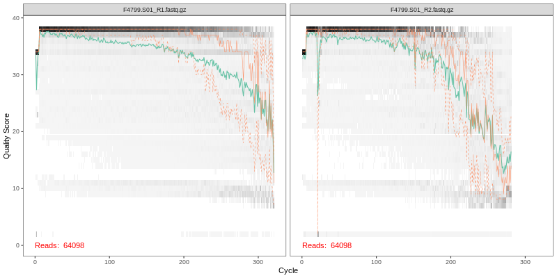
1. Read Quality Plots NGS sequence analaysis starts with visualizing the quality of the sequencing. Below are the quality plots of the first sample for the R1 and R2 reads separately. In gray-scale is a heat map of the frequency of each quality score at each base position. The mean quality score at each position is shown by the green line, and the quartiles of the quality score distribution by the orange lines. The forward reads are usually of better quality. It is a common practice to trim the last few nucleotides to avoid less well-controlled errors that can arise there. The trimming affects the downstream steps including error model building, merging and chimera calling. FOMC uses an empirical approach to test many combinations of different trim length in order to achieve best final amplicon sequence variants (ASVs), see the next section “Optimal trim length for ASVs”.

Below is the link to a PDF file for viewing the quality plots for all samples:

2. Optimal trim length for ASVs The final number of merged and chimera-filtered ASVs depends on the quality filtering (hence trimming) in the very beginning of the DADA2 pipeline. In order to achieve highest number of ASVs, an empirical approach was used -

1. Create a random subset of each sample consisting of 5,000 R1 and 5,000 R2 (to reduce computation time)
2. Trim 10 bases at a time from the ends of both R1 and R2 up to 50 bases
3. For each combination of trimmed length (e.g., 300x300, 300x290, 290x290 etc), the trimmed reads are subject to the entire DADA2 pipeline for chimera-filtered merged ASVs
4. The combination with highest percentage of the input reads becoming final ASVs is selected for the complete set of data

Below is the result of such operation, showing ASV percentages of total reads for all trimming combinations (1st Column = R1 lengths in bases; 1st Row = R2 lengths in bases):

Based on the above result, the trim length combination of R1 = 271 bases and R2 = 231 bases (highlighted red above), was chosen for generating final ASVs for all sequences. This combination generated highest number of merged non-chimeric ASVs and was used for downstream analyses, if requested.

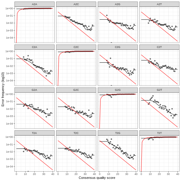
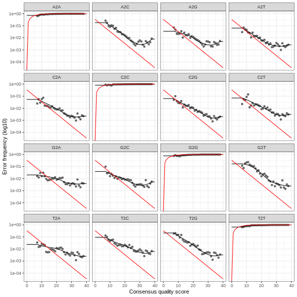
3. Error plots from learning the error rates After DADA2 building the error model for the set of data, it is always worthwhile, as a sanity check if nothing else, to visualize the estimated error rates. The error rates for each possible transition (A→C, A→G, …) are shown below. Points are the observed error rates for each consensus quality score. The black line shows the estimated error rates after convergence of the machine-learning algorithm. The red line shows the error rates expected under the nominal definition of the Q-score. The ideal result would be the estimated error rates (black line) are a good fit to the observed rates (points), and the error rates drop with increased quality as expected.

Forward Read R1 Error Plot


Reverse Read R2 Error Plot

The PDF version of these plots are available here:

4. DADA2 Result Summary The table below shows the summary of the DADA2 analysis, tracking paired read counts of each samples for all the steps during DADA2 denoising process - including end-trimming (filtered), denoising (denoisedF, denoisedF), pair merging (merged) and chimera removal (nonchim).

This table can be downloaded as an Excel table below:

5. DADA2 Amplicon Sequence Variants (ASVs). A total of 1050 unique merged and chimera-free ASV sequences were identified, and their corresponding read counts for each sample are available in the "ASV Read Count Table" with rows for the ASV sequences and columns for sample. This read count table can be used for microbial profile comparison among different samples and the sequences provided in the table can be used to taxonomy assignment.

The table can be downloaded from this link: