Project FOMC4038 services include NGS sequencing of the V1V3 region of the 16S rRNA amplicons from the samples. First and foremost, please
download this report, as well as the sequence raw data from the download links provided below.
These links will expire after 60 days. We cannot guarantee the availability of your data after 60 days.
Full Bioinformatics analysis service was requested. We provide many analyses, starting from the raw sequence quality and noise filtering, pair reads merging, as well as chimera filtering for the sequences, using the
DADA2 denosing algorithm and pipeline.
We also provide many downstream analyses such as taxonomy assignment, alpha and beta diversity analyses, and differential abundance analysis.
For taxonomy assignment, most informative would be the taxonomy barplots. We provide an interactive barplots to show the relative abundance of microbes at different taxonomy levels (from Phylum to species) that you can choose.
If you specify which groups of samples you want to compare for differential abundance, we provide both ANCOM and LEfSe differential abundance analysis.
The samples were processed and analyzed with the ZymoBIOMICS® Service: Targeted
Metagenomic Sequencing (Zymo Research, Irvine, CA).
DNA Extraction: If DNA extraction was performed, one of three different DNA
extraction kits was used depending on the sample type and sample volume and were
used according to the manufacturer’s instructions, unless otherwise stated. The kit used
in this project is marked below:
☐
ZymoBIOMICS® DNA Miniprep Kit (Zymo Research, Irvine, CA)
☐
ZymoBIOMICS® DNA Microprep Kit (Zymo Research, Irvine, CA)
☐
ZymoBIOMICS®-96 MagBead DNA Kit (Zymo Research, Irvine, CA)
☑
N/A (DNA Extraction Not Performed)
Elution Volume: 50µL
Additional Notes: NA
Targeted Library Preparation: The DNA samples were prepared for targeted
sequencing with the Quick-16S™ NGS Library Prep Kit (Zymo Research, Irvine, CA).
These primers were custom designed by Zymo Research to provide the best coverage
of the 16S gene while maintaining high sensitivity. The primer sets used in this project
are marked below:
☐
Quick-16S™ Primer Set V1-V2 (Zymo Research, Irvine, CA)
☑
Quick-16S™ Primer Set V1-V3 (Zymo Research, Irvine, CA)
☐
Quick-16S™ Primer Set V3-V4 (Zymo Research, Irvine, CA)
☐
Quick-16S™ Primer Set V4 (Zymo Research, Irvine, CA)
☐
Quick-16S™ Primer Set V6-V8 (Zymo Research, Irvine, CA)
☐
Other: NA
Additional Notes: NA
The sequencing library was prepared using an innovative library preparation process in
which PCR reactions were performed in real-time PCR machines to control cycles and
therefore limit PCR chimera formation. The final PCR products were quantified with
qPCR fluorescence readings and pooled together based on equal molarity. The final
pooled library was cleaned up with the Select-a-Size DNA Clean & Concentrator™
(Zymo Research, Irvine, CA), then quantified with TapeStation® (Agilent Technologies,
Santa Clara, CA) and Qubit® (Thermo Fisher Scientific, Waltham, WA).
Control Samples: The ZymoBIOMICS® Microbial Community Standard (Zymo
Research, Irvine, CA) was used as a positive control for each DNA extraction, if
performed. The ZymoBIOMICS® Microbial Community DNA Standard (Zymo Research,
Irvine, CA) was used as a positive control for each targeted library preparation.
Negative controls (i.e. blank extraction control, blank library preparation control) were
included to assess the level of bioburden carried by the wet-lab process.
Sequencing: The final library was sequenced on Illumina® MiSeq™ with a V3 reagent kit
(600 cycles). The sequencing was performed with 10% PhiX spike-in.
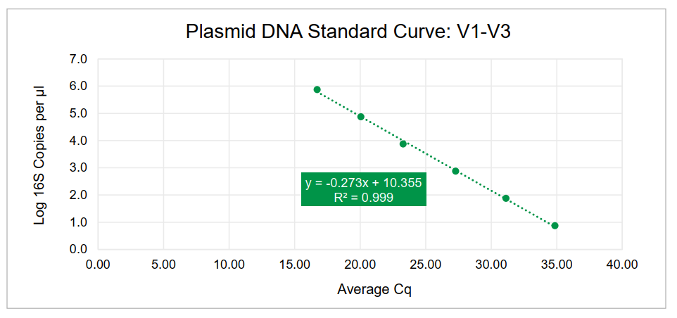
Absolute Abundance Quantification*: A quantitative real-time PCR was set up with a
standard curve. The standard curve was made with plasmid DNA containing one copy
of the 16S gene and one copy of the fungal ITS2 region prepared in 10-fold serial
dilutions. The primers used were the same as those used in Targeted Library
Preparation. The equation generated by the plasmid DNA standard curve was used to
calculate the number of gene copies in the reaction for each sample. The PCR input
volume (2 µl) was used to calculate the number of gene copies per microliter in each
DNA sample.
The number of genome copies per microliter DNA sample was calculated by dividing
the gene copy number by an assumed number of gene copies per genome. The value
used for 16S copies per genome is 4. The value used for ITS copies per genome is 200.
The amount of DNA per microliter DNA sample was calculated using an assumed
genome size of 4.64 x 10⁶ bp, the genome size of Escherichia coli, for 16S samples, or
an assumed genome size of 1.20 x 10⁷ bp, the genome size of Saccharomyces
cerevisiae, for ITS samples. This calculation is shown below:
Calculated Total DNA = Calculated Total Genome Copies × Assumed Genome Size (4.64 × 10⁶ bp) ×
Average Molecular Weight of a DNA bp (660 g/mole/bp) ÷ Avogadro’s Number (6.022 x 10²³/mole)
* Absolute Abundance Quantification is only available for 16S and ITS analyses.
The absolute abundance standard curve data can be viewed in Excel here:
The absolute abundance standard curve is shown below:
The complete report of your project, including all links in this report, can be downloaded by clicking the link provided below. The downloaded file is a compressed ZIP file and once unzipped, open the file “REPORT.html” (may only shown as "REPORT" in your computer) by double clicking it. Your default web browser will open it and you will see the exact content of this report.
Please download and save the file to your computer storage device. The download link will expire after 60 days upon your receiving of this report.
Complete report download link:
To view the report, please follow the following steps:
1.
Download the .zip file from the report link above.
2.
Extract all the contents of the downloaded .zip file to your desktop.
3.
Open the extracted folder and find the "REPORT.html" (may shown as only "REPORT").
4.
Open (double-clicking) the REPORT.html file. Your default browser will open the top age of the complete report. Within the
report, there are links to view all the analyses performed for the project.
The raw NGS sequence data is available for download with the link provided below. The data is a compressed ZIP file and can be unzipped to individual sequence files.
Since this is a pair-end sequencing, each of your samples is represented by two sequence files, one for READ 1,
with the file extension “*_R1.fastq.gz”, another READ 2, with the file extension “*_R1.fastq.gz”.
The files are in FASTQ format and are compressed. FASTQ format is a text-based data format for storing both a biological sequence
and its corresponding quality scores. Most sequence analysis software will be able to open them.
The Sample IDs associated with the R1 and R2 fastq files are listed in the table below:
Sample ID
Read 1 File Name
R1 Read Count
S10
zr4038_10V1V3_R1.fastq.gz
21847
S11
zr4038_11V1V3_R1.fastq.gz
24362
S12
zr4038_12V1V3_R1.fastq.gz
26032
S13
zr4038_13V1V3_R1.fastq.gz
25863
S14
zr4038_14V1V3_R1.fastq.gz
27704
S15
zr4038_15V1V3_R1.fastq.gz
25729
S16
zr4038_16V1V3_R1.fastq.gz
24525
S17
zr4038_17V1V3_R1.fastq.gz
34453
S18
zr4038_18V1V3_R1.fastq.gz
33123
S19
zr4038_19V1V3_R1.fastq.gz
26219
S01
zr4038_1V1V3_R1.fastq.gz
24835
S20
zr4038_20V1V3_R1.fastq.gz
31434
S21
zr4038_21V1V3_R1.fastq.gz
40154
S22
zr4038_22V1V3_R1.fastq.gz
32032
S23
zr4038_23V1V3_R1.fastq.gz
32991
S24
zr4038_24V1V3_R1.fastq.gz
28955
S25
zr4038_25V1V3_R1.fastq.gz
28979
S26
zr4038_26V1V3_R1.fastq.gz
30111
S27
zr4038_27V1V3_R1.fastq.gz
31544
S28
zr4038_28V1V3_R1.fastq.gz
24284
S29
zr4038_29V1V3_R1.fastq.gz
36452
S02
zr4038_2V1V3_R1.fastq.gz
26023
S30
zr4038_30V1V3_R1.fastq.gz
29563
S31
zr4038_31V1V3_R1.fastq.gz
37915
S32
zr4038_32V1V3_R1.fastq.gz
27783
S33
zr4038_33V1V3_R1.fastq.gz
27480
S34
zr4038_34V1V3_R1.fastq.gz
27440
S35
zr4038_35V1V3_R1.fastq.gz
24686
S36
zr4038_36V1V3_R1.fastq.gz
29049
S37
zr4038_37V1V3_R1.fastq.gz
40510
S38
zr4038_38V1V3_R1.fastq.gz
28569
S39
zr4038_39V1V3_R1.fastq.gz
29432
S03
zr4038_3V1V3_R1.fastq.gz
22346
S40
zr4038_40V1V3_R1.fastq.gz
25534
S41
zr4038_41V1V3_R1.fastq.gz
26940
S42
zr4038_42V1V3_R1.fastq.gz
24328
S43
zr4038_43V1V3_R1.fastq.gz
26032
S44
zr4038_44V1V3_R1.fastq.gz
31576
S45
zr4038_45V1V3_R1.fastq.gz
46498
S46
zr4038_46V1V3_R1.fastq.gz
29218
S47
zr4038_47V1V3_R1.fastq.gz
32764
S48
zr4038_48V1V3_R1.fastq.gz
24805
S49
zr4038_49V1V3_R1.fastq.gz
28827
S04
zr4038_4V1V3_R1.fastq.gz
23991
S50
zr4038_50V1V3_R1.fastq.gz
22762
S51
zr4038_51V1V3_R1.fastq.gz
12488
S52
zr4038_52V1V3_R1.fastq.gz
20212
S53
zr4038_53V1V3_R1.fastq.gz
29756
S54
zr4038_54V1V3_R1.fastq.gz
27982
S55
zr4038_55V1V3_R1.fastq.gz
27158
S56
zr4038_56V1V3_R1.fastq.gz
23374
S57
zr4038_57V1V3_R1.fastq.gz
16807
S58
zr4038_58V1V3_R1.fastq.gz
1324
S59
zr4038_59V1V3_R1.fastq.gz
23295
S05
zr4038_5V1V3_R1.fastq.gz
28359
S60
zr4038_60V1V3_R1.fastq.gz
22703
S61
zr4038_61V1V3_R1.fastq.gz
25310
S62
zr4038_62V1V3_R1.fastq.gz
23687
S63
zr4038_63V1V3_R1.fastq.gz
27268
S64
zr4038_64V1V3_R1.fastq.gz
30587
S65
zr4038_65V1V3_R1.fastq.gz
28561
S66
zr4038_66V1V3_R1.fastq.gz
28417
S67
zr4038_67V1V3_R1.fastq.gz
28530
S68
zr4038_68V1V3_R1.fastq.gz
33017
S69
zr4038_69V1V3_R1.fastq.gz
35383
S06
zr4038_6V1V3_R1.fastq.gz
24331
S70
zr4038_70V1V3_R1.fastq.gz
32626
S71
zr4038_71V1V3_R1.fastq.gz
28484
S72
zr4038_72V1V3_R1.fastq.gz
28371
S73
zr4038_73V1V3_R1.fastq.gz
23645
S74
zr4038_74V1V3_R1.fastq.gz
17486
S75
zr4038_75V1V3_R1.fastq.gz
16440
S76
zr4038_76V1V3_R1.fastq.gz
1197
S77
zr4038_77V1V3_R1.fastq.gz
20999
S78
zr4038_78V1V3_R1.fastq.gz
18748
S07
zr4038_7V1V3_R1.fastq.gz
27253
S08
zr4038_8V1V3_R1.fastq.gz
24716
S09
zr4038_9V1V3_R1.fastq.gz
25264
Please download and save the file to your computer storage device. The download link will expire after 60 days upon your receiving of this report.
DADA2 is a software package that models and corrects Illumina-sequenced amplicon errors.
DADA2 infers sample sequences exactly, without coarse-graining into OTUs,
and resolves differences of as little as one nucleotide. DADA2 identified more real variants
and output fewer spurious sequences than other methods.
DADA2’s advantage is that it uses more of the data. The DADA2 error model incorporates quality information,
which is ignored by all other methods after filtering. The DADA2 error model incorporates quantitative abundances,
whereas most other methods use abundance ranks if they use abundance at all.
The DADA2 error model identifies the differences between sequences, eg. A->C,
whereas other methods merely count the mismatches. DADA2 can parameterize its error model from the data itself,
rather than relying on previous datasets that may or may not reflect the PCR and sequencing protocols used in your study.
DADA2 pipeline includes several tools for read quality control, including quality filtering, trimming, denoising, pair merging and chimera filtering. Below are the major processing steps of DADA2:
Step 1. Read trimming based on sequence quality
The quality of NGS Illumina sequences often decreases toward the end of the reads.
DADA2 allows to trim off the poor quality read ends in order to improve the error
model building and pair merging performance.
Step 2. Learn the Error Rates
The DADA2 algorithm makes use of a parametric error model (err) and every
amplicon dataset has a different set of error rates. The learnErrors method
learns this error model from the data, by alternating estimation of the error
rates and inference of sample composition until they converge on a jointly
consistent solution. As in many machine-learning problems, the algorithm must
begin with an initial guess, for which the maximum possible error rates in
this data are used (the error rates if only the most abundant sequence is
correct and all the rest are errors).
Step 3. Infer amplicon sequence variants (ASVs) based on the error model built in previous step. This step is also called sequence "denoising".
The outcome of this step is a list of ASVs that are the equivalent of oligonucleotides.
Step 4. Merge paired reads. If the sequencing products are read pairs, DADA2 will merge the R1 and R2 ASVs into single sequences.
Merging is performed by aligning the denoised forward reads with the reverse-complement of the corresponding
denoised reverse reads, and then constructing the merged “contig” sequences.
By default, merged sequences are only output if the forward and reverse reads overlap by
at least 12 bases, and are identical to each other in the overlap region (but these conditions can be changed via function arguments).
Step 5. Remove chimera.
The core dada method corrects substitution and indel errors, but chimeras remain. Fortunately, the accuracy of sequence variants
after denoising makes identifying chimeric ASVs simpler than when dealing with fuzzy OTUs.
Chimeric sequences are identified if they can be exactly reconstructed by
combining a left-segment and a right-segment from two more abundant “parent” sequences. The frequency of chimeric sequences varies substantially
from dataset to dataset, and depends on on factors including experimental procedures and sample complexity.
Results
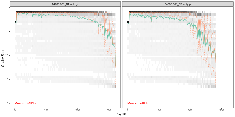
1. Read Quality Plots NGS sequence analysis starts with visualizing the quality of the sequencing. Below are the quality plots of the first
sample for the R1 and R2 reads separately. In gray-scale is a heat map of the frequency of each quality score at each base position. The mean
quality score at each position is shown by the green line, and the quartiles of the quality score distribution by the orange lines.
The forward reads are usually of better quality. It is a common practice to trim the last few nucleotides to avoid less well-controlled errors
that can arise there. The trimming affects the downstream steps including error model building, merging and chimera calling. FOMC uses an empirical
approach to test many combinations of different trim length in order to achieve best final amplicon sequence variants (ASVs), see the next
section “Optimal trim length for ASVs”.
Below is the link to a PDF file for viewing the quality plots for all samples:
2. Optimal trim length for ASVs The final number of merged and chimera-filtered ASVs depends on the quality filtering (hence trimming) in the very beginning of the DADA2 pipeline.
In order to achieve highest number of ASVs, an empirical approach was used -
Create a random subset of each sample consisting of 5,000 R1 and 5,000 R2 (to reduce computation time)
Trim 10 bases at a time from the ends of both R1 and R2 up to 50 bases
For each combination of trimmed length (e.g., 300x300, 300x290, 290x290 etc), the trimmed reads are
subject to the entire DADA2 pipeline for chimera-filtered merged ASVs
The combination with highest percentage of the input reads becoming final ASVs is selected for the complete set of data
Below is the result of such operation, showing ASV percentages of total reads for all trimming combinations (1st Column = R1 lengths in bases; 1st Row = R2 lengths in bases):
R1/R2
281
271
261
251
241
231
321
31.02%
41.32%
41.86%
42.65%
43.40%
39.58%
311
34.37%
45.49%
45.98%
46.56%
43.95%
34.08%
301
34.96%
45.82%
46.41%
42.90%
34.03%
21.86%
291
34.86%
45.53%
42.34%
32.96%
21.99%
16.04%
281
34.82%
41.74%
33.08%
21.36%
16.00%
8.20%
271
31.72%
32.97%
21.34%
15.72%
8.28%
5.02%
Based on the above result, the trim length combination of R1 = 311 bases and R2 = 251 bases (highlighted red above), was chosen for generating final ASVs for all sequences.
This combination generated highest number of merged non-chimeric ASVs and was used for downstream analyses, if requested.
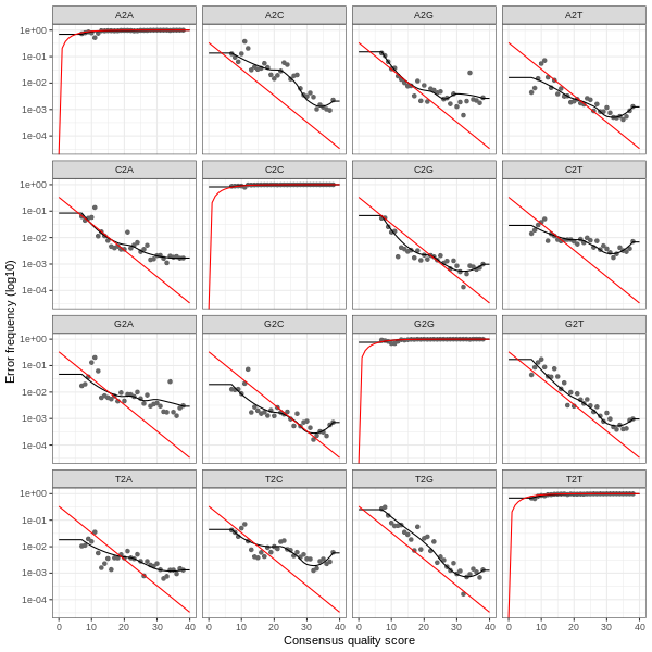
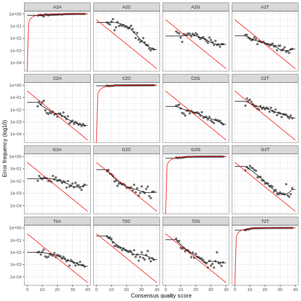
3. Error plots from learning the error rates
After DADA2 building the error model for the set of data, it is always worthwhile, as a sanity check if nothing else, to visualize the estimated error rates.
The error rates for each possible transition (A→C, A→G, …) are shown below. Points are the observed error rates for each consensus quality score.
The black line shows the estimated error rates after convergence of the machine-learning algorithm.
The red line shows the error rates expected under the nominal definition of the Q-score.
The ideal result would be the estimated error rates (black line) are a good fit to the observed rates (points), and the error rates drop
with increased quality as expected.
Forward Read R1 Error Plot
Reverse Read R2 Error Plot
The PDF version of these plots are available here:
4. DADA2 Result Summary The table below shows the summary of the DADA2 analysis,
tracking paired read counts of each samples for all the steps during DADA2 denoising process -
including end-trimming (filtered), denoising (denoisedF, denoisedF), pair merging (merged) and chimera removal (nonchim).
Sample ID
F4038.S01
F4038.S02
F4038.S03
F4038.S04
F4038.S05
F4038.S06
F4038.S07
F4038.S08
F4038.S09
F4038.S10
F4038.S11
F4038.S12
F4038.S13
F4038.S14
F4038.S15
F4038.S16
F4038.S17
F4038.S18
F4038.S19
F4038.S20
F4038.S21
F4038.S22
F4038.S23
F4038.S24
F4038.S25
F4038.S26
F4038.S27
F4038.S28
F4038.S29
F4038.S30
F4038.S31
F4038.S32
F4038.S33
F4038.S34
F4038.S35
F4038.S36
F4038.S37
F4038.S38
F4038.S39
F4038.S40
F4038.S41
F4038.S42
F4038.S43
F4038.S44
F4038.S45
F4038.S46
F4038.S47
F4038.S48
F4038.S49
F4038.S50
F4038.S51
F4038.S52
F4038.S53
F4038.S54
F4038.S55
F4038.S56
F4038.S57
F4038.S58
F4038.S59
F4038.S60
F4038.S61
F4038.S62
F4038.S63
F4038.S64
F4038.S65
F4038.S66
F4038.S67
F4038.S68
F4038.S69
F4038.S70
F4038.S71
F4038.S72
F4038.S73
F4038.S74
F4038.S75
F4038.S76
F4038.S77
F4038.S78
Row Sum
Percentage
input
24,835
26,023
22,346
23,991
28,359
24,331
27,253
24,716
25,264
21,847
24,362
26,032
25,863
27,704
25,729
24,525
34,453
33,123
26,219
31,434
40,154
32,032
32,991
28,955
28,979
30,111
31,544
24,284
36,452
29,563
37,915
27,783
27,480
27,440
24,686
29,049
40,510
28,569
29,432
25,534
26,940
24,328
26,032
31,576
46,498
29,218
32,764
24,805
28,827
22,762
12,488
20,212
29,756
27,982
27,158
23,374
16,807
1,324
23,295
22,703
25,310
23,687
27,268
30,587
28,561
28,417
28,530
33,017
35,383
32,626
28,484
28,371
23,645
17,486
16,440
1,197
20,999
18,748
2,089,477
100.00%
filtered
18,709
20,107
16,369
18,390
21,792
17,903
20,629
19,109
18,636
16,220
18,064
19,955
19,777
20,531
18,706
18,547
26,217
26,465
19,445
22,371
31,417
24,690
25,924
22,016
22,124
23,443
24,153
18,772
27,561
22,652
29,418
21,469
20,589
20,917
18,353
22,017
29,868
21,154
21,326
19,269
20,309
18,716
19,995
22,627
35,832
22,054
24,946
19,360
21,708
17,272
796
15,347
23,175
19,881
20,128
18,138
10,771
170
18,168
17,238
20,090
17,379
20,337
23,501
21,262
22,483
22,319
25,284
27,348
25,103
21,889
21,522
17,886
13,330
12,030
207
16,378
14,116
1,574,169
75.34%
denoisedF
18,047
19,187
15,763
17,536
20,956
17,253
19,985
18,022
17,815
15,491
17,447
19,131
18,841
19,513
17,933
17,862
25,427
25,454
18,870
21,772
30,521
23,562
24,999
21,471
21,164
22,443
23,252
17,672
26,493
21,300
28,219
20,442
19,550
20,411
17,495
21,536
29,138
20,211
20,448
18,557
19,614
18,113
18,964
21,903
34,608
21,097
23,882
18,672
20,568
16,060
608
14,543
21,995
19,231
19,672
17,243
10,242
159
17,165
16,724
19,259
16,668
19,597
22,863
20,528
21,798
21,473
24,650
26,381
24,212
21,110
20,572
16,947
12,738
11,657
131
15,416
13,520
1,511,772
72.35%
denoisedR
18,341
19,428
15,855
17,808
20,971
17,390
20,080
18,266
18,042
15,666
17,497
19,393
18,990
19,969
18,210
18,013
25,676
25,710
19,014
21,846
30,763
23,738
25,288
21,744
21,165
22,876
23,582
18,058
26,723
21,791
28,639
20,872
20,006
20,298
17,921
21,674
29,586
20,469
20,349
18,752
19,723
18,061
19,507
22,229
34,851
21,083
24,174
18,887
20,839
16,470
708
14,047
22,508
19,449
19,916
17,260
10,054
159
17,320
16,882
19,380
16,909
19,891
23,141
20,710
21,894
21,583
24,948
26,771
24,367
21,317
20,889
17,382
13,013
11,825
140
15,589
13,534
1,527,869
73.12%
merged
16,027
17,464
13,057
15,428
18,532
15,135
17,630
15,200
15,641
13,384
15,009
16,512
15,499
17,254
14,732
15,590
23,240
21,780
16,489
19,073
27,287
19,793
21,541
19,881
17,975
19,681
19,885
13,922
22,783
17,560
24,246
18,223
16,335
18,221
15,241
20,166
27,523
17,970
17,046
16,459
17,388
16,455
16,481
19,599
31,444
17,845
20,333
15,672
17,075
13,715
566
11,254
17,890
15,902
18,595
13,011
7,529
0
14,600
15,165
16,659
14,575
17,459
21,702
18,295
19,448
18,592
22,990
23,902
21,143
18,552
18,059
15,325
11,724
10,979
129
12,922
11,517
1,318,905
63.12%
nonchim
9,152
9,745
7,385
7,854
9,821
8,330
8,444
8,194
8,661
7,391
8,362
8,513
9,394
9,378
7,323
6,364
10,682
9,333
7,808
9,814
13,487
9,125
9,288
9,561
10,557
9,856
10,443
7,915
13,822
9,740
11,773
9,448
8,755
7,386
8,497
9,712
16,966
10,271
9,531
8,246
7,956
8,515
8,012
10,525
17,237
9,606
12,464
7,512
9,773
9,087
338
5,729
7,362
7,685
11,551
5,595
4,146
0
8,831
7,045
10,799
6,756
9,890
10,356
11,484
9,148
8,931
14,857
11,323
10,589
8,416
8,961
7,432
5,162
4,172
129
7,271
6,586
687,558
32.91%
This table can be downloaded as an Excel table below:
5. DADA2 Amplicon Sequence Variants (ASVs). A total of 15440 unique merged and chimera-free ASV sequences were identified, and their corresponding
read counts for each sample are available in the "ASV Read Count Table" with rows for the ASV sequences and columns for sample. This read count table can be used for
microbial profile comparison among different samples and the sequences provided in the table can be used to taxonomy assignment.
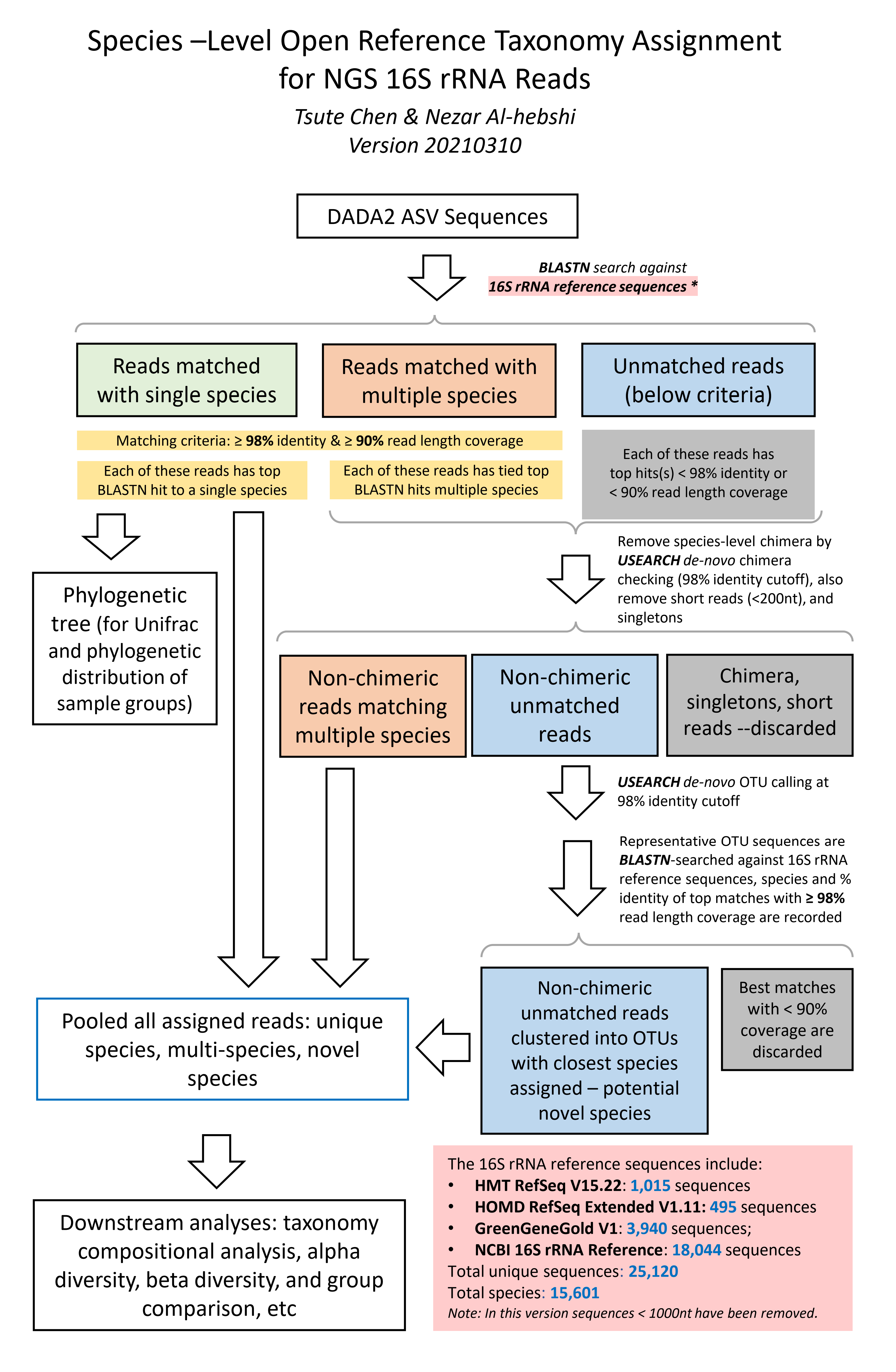
The species-level, open-reference 16S rRNA NGS reads taxonomy assignment pipeline
Version 20210310
1. Raw sequences reads in FASTA format were BLASTN-searched against a combined set of 16S rRNA reference sequences.
It consists of MOMD (version 0.1), the HOMD (version 15.2 http://www.homd.org/index.php?name=seqDownload&file&type=R ),
HOMD 16S rRNA RefSeq Extended Version 1.1 (EXT), GreenGene Gold (GG)
(http://greengenes.lbl.gov/Download/Sequence_Data/Fasta_data_files/gold_strains_gg16S_aligned.fasta.gz) ,
and the NCBI 16S rRNA reference sequence set (https://ftp.ncbi.nlm.nih.gov/blast/db/16S_ribosomal_RNA.tar.gz).
These sequences were screened and combined to remove short sequences (<1000nt), chimera, duplicated and sub-sequences,
as well as sequences with poor taxonomy annotation (e.g., without species information).
This process resulted in 1,015 from HOMD V15.22, 495 from EXT, 3,940 from GG and 18,044 from NCBI, a total of 25,120 sequences.
Altogether these sequences represent a total of 15,601 oral and non-oral microbial species.
The NCBI BLASTN version 2.7.1+ (Zhang et al, 2000) was used with the default parameters.
Reads with ≥ 98% sequence identity to the matched reference and ≥ 90% alignment length
(i.e., ≥ 90% of the read length that was aligned to the reference and was used to calculate
the sequence percent identity) were classified based on the taxonomy of the reference sequence
with highest sequence identity. If a read matched with reference sequences representing
more than one species with equal percent identity and alignment length, it was subject
to chimera checking with USEARCH program version v8.1.1861 (Edgar 2010). Non-chimeric reads with multi-species
best hits were considered valid and were assigned with a unique species
notation (e.g., spp) denoting unresolvable multiple species.
2. Unassigned reads (i.e., reads with < 98% identity or < 90% alignment length) were pooled together and reads < 200 bases were
removed. The remaining reads were subject to the de novo
operational taxonomy unit (OTU) calling and chimera checking using the USEARCH program version v8.1.1861 (Edgar 2010).
The de novo OTU calling and chimera checking was done using 98% as the sequence identity cutoff, i.e., the species-level OTU.
The output of this step produced species-level de novo clustered OTUs with 98% identity.
Representative reads from each of the OTUs/species were then BLASTN-searched
against the same reference sequence set again to determine the closest species for
these potential novel species. These potential novel species were pooled together with the reads that were signed to specie-level in
the previous step, for down-stream analyses.
Reference:
Edgar RC. Search and clustering orders of magnitude faster than BLAST.
Bioinformatics. 2010 Oct 1;26(19):2460-1. doi: 10.1093/bioinformatics/btq461. Epub 2010 Aug 12. PubMed PMID: 20709691.
3. Designations used in the taxonomy:
	1) Taxonomy levels are indicated by these prefixes:

	   k__: domain/kingdom
	   p__: phylum
	   c__: class
	   o__: order
	   f__: family
	   g__: genus
	   s__: species

	   Example:

	   k__Bacteria;p__Firmicutes;c__Clostridia;o__Clostridiales;f__Lachnospiraceae;g__Blautia;s__faecis

	2) Unique level identified – known species:

	   k__Bacteria;p__Firmicutes;c__Clostridia;o__Clostridiales;f__Lachnospiraceae;g__Roseburia;s__hominis

	   The above example shows some reads match to a single species (all levels are unique)

	3) Non-unique level identified – known species:

	   k__Bacteria;p__Firmicutes;c__Clostridia;o__Clostridiales;f__Lachnospiraceae;g__Roseburia;s__multispecies_spp123_3

	   The above example “s__multispecies_spp123_3” indicates certain reads equally match to 3 species of the
	   genus Roseburia; the “spp123” is a temporally assigned species ID.

	   k__Bacteria;p__Firmicutes;c__Clostridia;o__Clostridiales;f__Lachnospiraceae;g__multigenus;s__multispecies_spp234_5

	   The above example indicates certain reads match equally to 5 different species, which belong to multiple genera.;
	   the “spp234” is a temporally assigned species ID.

	4) Unique level identified – unknown species, potential novel species:

	   k__Bacteria;p__Firmicutes;c__Clostridia;o__Clostridiales;f__Lachnospiraceae;g__Roseburia;s__ hominis_nov_97%

	   The above example indicates that some reads have no match to any of the reference sequences with
	   sequence identity ≥ 98% and percent coverage (alignment length)  ≥ 98% as well. However this groups
	   of reads (actually the representative read from a de novo  OTU) has 96% percent identity to
	   Roseburia hominis, thus this is a potential novel species, closest to Roseburia hominis.
	   (But they are not the same species).

	5) Multiple level identified – unknown species, potential novel species:
	   k__Bacteria;p__Firmicutes;c__Clostridia;o__Clostridiales;f__Lachnospiraceae;g__Roseburia;s__ multispecies_sppn123_3_nov_96%

	   The above example indicates that some reads have no match to any of the reference sequences
	   with sequence identity ≥ 98% and percent coverage (alignment length)  ≥ 98% as well.
	   However this groups of reads (actually the representative read from a de novo  OTU)
	   has 96% percent identity equally to 3 species in Roseburia. Thus this is no single
	   closest species, instead this group of reads match equally to multiple species at 96%.
	   Since they have passed chimera check so they represent a novel species. “sppn123” is a
	   temporary ID for this potential novel species.
4. The taxonomy assignment algorithm is illustrated in this flow chart below:
Read Taxonomy Assignment - Result Summary
Code
Category
Read Count (MC=1)*
Read Count (MC=100)*
A
Total reads
687,558
687,558
B
Total assigned reads
685,541
685,541
C
Assigned reads in species with read count < MC
0
11,645
D
Assigned reads in samples with read count < 500
467
467
E
Total samples
77
77
F
Samples with reads >= 500
75
75
G
Samples with reads < 500
2
2
H
Total assigned reads used for analysis (B-C-D)
685,074
673,429
I
Reads assigned to single species
655,452
649,782
J
Reads assigned to multiple species
17,817
16,452
K
Reads assigned to novel species
11,805
7,195
L
Total number of species
737
364
M
Number of single species
458
316
N
Number of multi-species
44
15
O
Number of novel species
235
33
P
Total unassigned reads
2,017
2,017
Q
Chimeric reads
262
262
R
Reads without BLASTN hits
23
23
S
Others: short, low quality, singletons, etc.
1,732
1,732
A=B+P=C+D+H+Q+R+S
E=F+G
B=C+D+H
H=I+J+K
L=M+N+O
P=Q+R+S
* MC = Minimal Count per species, species with total read count < MC were removed.
* The assignment result from MC=100 was used in the downstream analyses.
Read Taxonomy Assignment - Sample Meta Information
#SampleID
Sample_name
visit
icam_change
vcam_change
perio
F4038.S01
1001.BS.1
Visit 1
Decrease
Decrease
Yes
F4038.S02
15.BS.2
Visit 1
Increase
Increase
No
F4038.S03
21.BS.3
Visit 1
Decrease
Increase
No
F4038.S04
266.BS.4
Visit 1
Increase
Increase
No
F4038.S05
43.BS.5
Visit 1
Decrease
Decrease
Yes
F4038.S06
52.BS.6
Visit 1
Increase
Increase
Yes
F4038.S07
59.BS.7
Visit 1
Decrease
Decrease
No
F4038.S08
106.BS.8
Visit 1
Decrease
Decrease
Yes
F4038.S09
126.BS.9
Visit 1
Decrease
Increase
Yes
F4038.S10
144.BS.10
Visit 1
Increase
Decrease
No
F4038.S11
188.BS.11
Visit 1
Increase
Decrease
No
F4038.S12
873.BS.12
Visit 1
Decrease
Increase
Yes
F4038.S13
1027.BS.13
Visit 1
Decrease
Decrease
Yes
F4038.S14
908.BS.14
Visit 1
Decrease
Decrease
Yes
F4038.S15
938.BS.15
Visit 1
Decrease
Increase
No
F4038.S16
729.BS.16
Visit 1
Increase
Increase
Yes
F4038.S17
601.BS.17
Visit 1
Decrease
Increase
No
F4038.S18
629.BS.18
Visit 1
Decrease
Decrease
Yes
F4038.S19
63.BS.19
Visit 1
Decrease
Increase
No
F4038.S20
582.BS.20
Visit 1
Increase
Increase
No
F4038.S21
452.BS.21
Visit 1
Increase
Increase
No
F4038.S22
508.BS.23
Visit 1
Increase
Increase
No
F4038.S23
564.BS.24
Visit 1
Decrease
Decrease
Yes
F4038.S24
238.BS.25
Visit 1
Increase
Increase
No
F4038.S25
618.BS.26
Visit 1
Increase
Increase
No
F4038.S26
680.BS.28
Visit 1
Decrease
Increase
Yes
F4038.S27
691.BS.29
Visit 1
Increase
Increase
Yes
F4038.S28
696.BS.30
Visit 1
Increase
Increase
Yes
F4038.S29
717.BS.31
Visit 1
Increase
Increase
Yes
F4038.S30
790.BS.32
Visit 1
Decrease
Decrease
Yes
F4038.S31
803.BS.33
Visit 1
Decrease
Decrease
Yes
F4038.S32
807.BS.34
Visit 1
Increase
Increase
No
F4038.S33
824.BS.35
Visit 1
Increase
Increase
Yes
F4038.S34
831.BS.36
Visit 1
Increase
Increase
No
F4038.S35
870.BS.37
Visit 1
Increase
Decrease
Yes
F4038.S36
282.BS.38
Visit 1
Increase
Increase
No
F4038.S37
317.BS.39
Visit 1
Decrease
Decrease
No
F4038.S38
403.BS.40
Visit 1
Decrease
Decrease
No
F4038.S39
433.BS.41
Visit 1
Decrease
Decrease
No
F4038.S40
1001.V2.42
Visit 2
Decrease
Decrease
Yes
F4038.S41
15.V2.43
Visit 2
Increase
Increase
No
F4038.S42
43.V2.44
Visit 2
Decrease
Decrease
Yes
F4038.S43
266.V2.45
Visit 2
Increase
Increase
No
F4038.S44
52.V2.46
Visit 2
Increase
Increase
Yes
F4038.S45
106.V2.47
Visit 2
Decrease
Decrease
Yes
F4038.S46
21.V2.48
Visit 2
Decrease
Increase
No
F4038.S47
188.V2.49
Visit 2
Increase
Decrease
No
F4038.S48
59.V2.50
Visit 2
Decrease
Decrease
No
F4038.S49
126.V2.51
Visit 2
Decrease
Increase
Yes
F4038.S50
144.V2.52
Visit 2
Increase
Decrease
No
F4038.S51
282.V2.53
Visit 2
Increase
Increase
No
F4038.S52
403.V2.54
Visit 2
Decrease
Decrease
No
F4038.S53
452.V2.55
Visit 2
Increase
Increase
No
F4038.S54
582.V2.56
Visit 2
Increase
Increase
No
F4038.S55
317.V2.57
Visit 2
Decrease
Decrease
No
F4038.S56
508.V2.58
Visit 2
Increase
Increase
No
F4038.S57
564.V2.59
Visit 2
Decrease
Decrease
Yes
F4038.S58
601.V2.60
Visit 2
Decrease
Increase
No
F4038.S59
629.V2.62
Visit 2
Decrease
Decrease
Yes
F4038.S60
680.V2.63
Visit 2
Decrease
Increase
Yes
F4038.S61
696.V2.64
Visit 2
Increase
Increase
Yes
F4038.S62
717.V2.65
Visit 2
Increase
Increase
Yes
F4038.S63
790.V2.66
Visit 2
Decrease
Decrease
Yes
F4038.S64
803.V2.67
Visit 2
Decrease
Decrease
Yes
F4038.S65
618.V2.68
Visit 2
Increase
Increase
No
F4038.S66
831.V2.69
Visit 2
Increase
Increase
No
F4038.S67
691.V2.70
Visit 2
Increase
Increase
Yes
F4038.S68
873.V2.71
Visit 2
Decrease
Increase
Yes
F4038.S69
908.V2.72
Visit 2
Decrease
Decrease
Yes
F4038.S70
938.V2.73
Visit 2
Decrease
Increase
No
F4038.S71
807.V2.74
Visit 2
Increase
Increase
No
F4038.S72
729.V2.75
Visit 2
Increase
Increase
Yes
F4038.S73
1027.V2.76
Visit 2
Decrease
Decrease
Yes
F4038.S74
870.V2.77
Visit 2
Increase
Decrease
Yes
F4038.S75
63.V2.78
Visit 2
Decrease
Increase
No
F4038.S76
433.V2.79
Visit 2
Decrease
Decrease
No
F4038.S77
824.V2.80
Visit 2
Increase
Increase
Yes
F4038.S78
238.V2.81
Visit 2
Increase
Increase
No
Read Taxonomy Assignment - ASV Read Counts by Samples
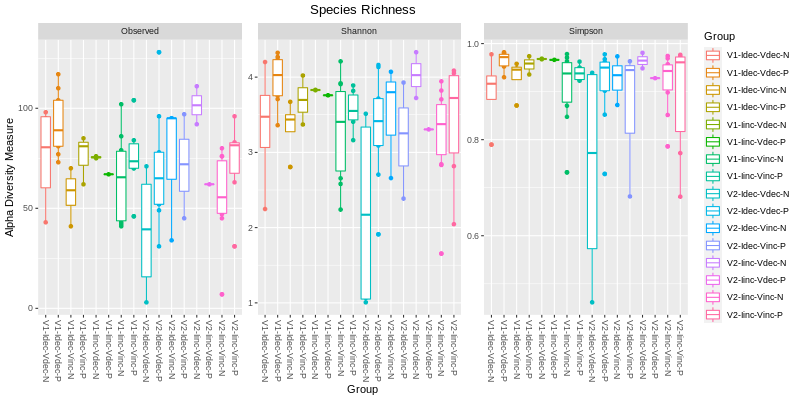
In ecology, alpha diversity (α-diversity) is the mean species diversity in sites or habitats at a local scale.
The term was introduced by R. H. Whittaker[1][2] together with the terms beta diversity (β-diversity)
and gamma diversity (γ-diversity). Whittaker's idea was that the total species diversity in a landscape
(gamma diversity) is determined by two different things, the mean species diversity in sites or habitats
at a more local scale (alpha diversity) and the differentiation among those habitats (beta diversity).
The two main factors taken into account when measuring diversity are richness and evenness.
Richness is a measure of the number of different kinds of organisms present in a particular area.
Evenness compares the similarity of the population size of each of the species present. There are
many different ways to measure the richness and evenness. These measurements are called "estimators" or "indices".
Below is a diversity of 3 commonly used indices showing the values for all the samples (dots) and in groups (boxes).
Alpha diversity analysis by rarefaction
Diversity measures are affected by the sampling depth. Rarefaction is a technique to assess species richness from the results of sampling. Rarefaction allows
the calculation of species richness for a given number of individual samples, based on the construction
of so-called rarefaction curves. This curve is a plot of the number of species as a function of the
number of samples. Rarefaction curves generally grow rapidly at first, as the most common species are found,
but the curves plateau as only the rarest species remain to be sampled.
Beta diversity compares the similarity (or dissimilarity) of microbial profiles between different
groups of samples. There are many different similarity/dissimilarity metrics.
In general, they can be quantitative (using sequence abundance, e.g., Bray-Curtis or weighted UniFrac)
or binary (considering only presence-absence of sequences, e.g., binary Jaccard or unweighted UniFrac).
They can be even based on phylogeny (e.g., UniFrac metrics) or not (non-UniFrac metrics, such as Bray-Curtis, etc.).
For microbiome studies, species profiles of samples can be compared with the Bray-Curtis dissimilarity,
which is based on the count data type. The pair-wise Bray-Curtis dissimilarity matrix of all samples can then be
subject to either multi-dimensional scaling (MDS, also known as PCoA) or non-metric MDS (NMDS).
MDS/PCoA is a
scaling or ordination method that starts with a matrix of similarities or dissimilarities
between a set of samples and aims to produce a low-dimensional graphical plot of the data
in such a way that distances between points in the plot are close to original dissimilarities.
NMDS is similar to MDS, however it does not use the dissimilarities data, instead it converts them into
the ranks and use these ranks in the calculation.
In our beta diversity analysis, Bray-Curtis dissimilarity matrix was first calculated and then plotted by the PCoA and
NMDS separately. The results are shown below:
The above PCoA and NMDS plots are based on count data. The count data can also be transformed into centered log ratio (CLR)
for each species. The CLR data is no longer count data and cannot be used in Bray-Curtis dissimilarity calculation. Instead
CLR can be compared with Euclidean distances. When CLR data are compared by Euclidean distance, the distance is also called
Aitchison distance.
Below are the NMDS and PCoA plots of the Aitchison distances of the samples:
Interactive 3D PCoA Plots - Bray-Curtis Dissimilarity
Interactive 3D PCoA Plots - Euclidean Distance
Interactive 3D PCoA Plots - Correlation Coefficients
16S rRNA next generation sequencing (NGS) generates a fixed number of reads that reflect the proportion of different species in a sample, i.e., the relative abundance of species, instead of the absolute abundance. In Mathematics, measurements involving probabilities, proportions, percentages, and ppm can all be thought of as compositional data. This makes the microbiome read count data “compositional” (Gloor et al, 2017). In general, compositional data represent parts of a whole which only carry relative information (http://www.compositionaldata.com/).
The problem of microbiome data being compositional arises when comparing two groups of samples for identifying “differentially abundant” species. A species with the same absolute abundance between two conditions, its relative abundances in the two conditions (e.g., percent abundance) can become different if the relative abundance of other species change greatly. This problem can lead to incorrect conclusion in terms of differential abundance for microbial species in the samples.
When studying differential abundance (DA), the current better approach is to transform the read count data into log ratio data. The ratios are calculated between read counts of all species in a sample to a “reference” count (e.g., mean read count of the sample). The log ratio data allow the detection of DA species without being affected by percentage bias mentioned above
In this report, a compositional DA analysis tool “ANCOM” (analysis of composition of microbiomes) was used. ANCOM transforms the count data into log-ratios and thus is more suitable for comparing the composition of microbiomes in two or more populations
References:
Gloor GB, Macklaim JM, Pawlowsky-Glahn V, Egozcue JJ. Microbiome Datasets Are Compositional: And This Is Not Optional. Front Microbiol.
2017 Nov 15;8:2224. doi: 10.3389/fmicb.2017.02224. PMID: 29187837; PMCID: PMC5695134.
Mandal S, Van Treuren W, White RA, Eggesbø M, Knight R, Peddada SD. Analysis of composition of
microbiomes: a novel method for studying microbial composition. Microb Ecol Health Dis.
2015 May 29;26:27663. doi: 10.3402/mehd.v26.27663. PMID: 26028277; PMCID: PMC4450248.
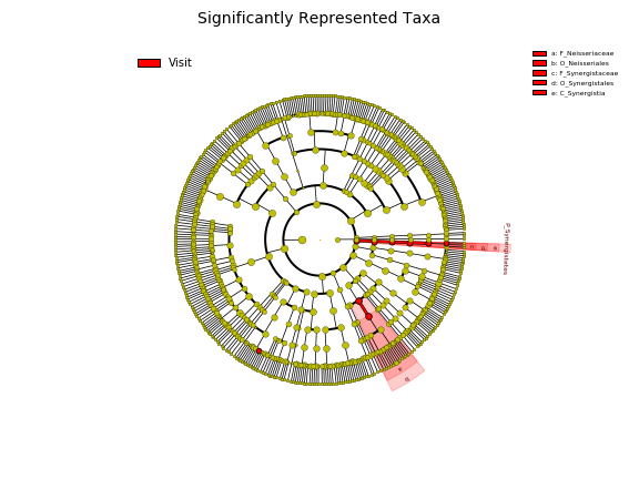
LEfSe (Linear Discriminant Analysis Effect Size) is an alternative method to find "organisms, genes, or
pathways that consistently explain the differences between two or more microbial communities" (Segata et al., 2011).
Specifically, LEfSe uses rank-based Kruskal-Wallis (KW) sum-rank test to detect features with significant
differential (relative) abundance with respect to the class of interest. Since it is rank-based, instead of proportional based,
the differential species identified among the comparison groups is less biased (than percent abundance based).
Reference:
Segata N, Izard J, Waldron L, Gevers D, Miropolsky L, Garrett WS, Huttenhower C. Metagenomic biomarker discovery and explanation. Genome Biol. 2011 Jun 24;12(6):R60. doi: 10.1186/gb-2011-12-6-r60. PMID: 21702898; PMCID: PMC3218848.
To analyze the co-occurrence or co-exclusion between microbial species among different samples, network correlation
analysis tools are usually used for this purpose. However, microbiome count data are compositional. If count data are normalized to the total number of counts in the
sample, the data become not independent and traditional statistical metrics (e.g., correlation) for the detection
of specie-species relationships can lead to spurious results. In addition, sequencing-based studies typically
measure hundreds of OTUs (species) on few samples; thus, inference of OTU-OTU association networks is severely
under-powered. Here we use SPIEC-EASI (SParse InversECovariance Estimation
for Ecological Association Inference), a statistical method for the inference of microbial
ecological networks from amplicon sequencing datasets that addresses both of these issues (Kurtz et al., 2015).
SPIEC-EASI combines data transformations developed for compositional data analysis with a graphical model
inference framework that assumes the underlying ecological association network is sparse. SPIEC-EASI provides
two algorithms for network inferencing – 1) Meinshausen-Bühlmann's neighborhood selection (MB method) and inverse covariance selection
(GLASSO method, i.e., graphical least absolute shrinkage and selection operator). This is fundamentally distinct from SparCC, which essentially estimate pairwise correlations. In addition
to these two methods, we provide the results of a third method - SparCC (Sparse Correlations for Compositional Data)(Friedman & Alm 2012), which
is also a method for inferring correlations from compositional data. SparCC estimates the linear Pearson correlations between
the log-transformed components.
References:
Kurtz ZD, Müller CL, Miraldi ER, Littman DR, Blaser MJ, Bonneau RA. Sparse and compositionally robust inference of microbial ecological networks. PLoS Comput Biol. 2015 May 7;11(5):e1004226. doi: 10.1371/journal.pcbi.1004226. PMID: 25950956; PMCID: PMC4423992.


